Euler method

For integrating with respect to the euler characteristic, see Euler calculus.

Not to be confused with Euler's factorization method.

In mathematics and computational science, the Euler method, named after Leonhard Euler, is a first-order numerical procedure for solving ordinary differential equations (ODEs) with a given initial value. It is the most basic kind of explicit method for numerical integration of ordinary differential equations and is the simplest kind of Runge-Kutta method.

1 Informal geometrical description
2 Derivation
3 Example
4 Error
5 Error bound
6 Numerical stability
7 See also
8 References
9 External links

Informal geometrical description

Consider the problem of calculating the shape of an unknown curve which starts at a given point and satisfies a given differential equation. Here, a differential equation can be thought of as a formula by which the slope of the tangent line to the curve can be computed at any point on the curve, once the position of that point has been calculated.

The idea is that while the curve is initially unknown, its starting point, which we denote by $A_0,$ is known (see the picture on top right). Then, from the differential equation, the slope to the curve at $A_0$ can be computed, and so, the tangent line.

Take a small step along that tangent line up to a point $A_1.$ If we pretend that $A_1$ is still on the curve, the same reasoning as for the point $A_0$ above can be used. After several steps, a polygonal curve $A_0A_1A_2A_3\dots$ is computed. In general, this curve does not diverge too far from the original unknown curve, and the error between the two curves can be made small if the step size is small enough and the interval of computation is finite (although things are more complicated for stiff equations, as discussed below).

Derivation

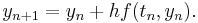
We want to approximate the solution of the initial value problem

$y'(t) = f(t,y(t)), \qquad \qquad y(t_0)=y_0,$

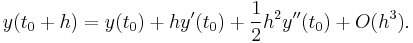
by using the first two terms of the Taylor expansion of y, which represents the linear approximation around the point (t₀,y(t₀)) . One step of the Euler method from t_n to t_n+1 = t_n + h is

$y_{n%2B1} = y_n %2B hf(t_n,y_n). \qquad \qquad$

The Euler method is explicit, i.e. the solution $y_{n%2B1}$ is an explicit function of $y_i$ for $i \leq n$ .

While the Euler method integrates a first order ODE, any ODE of order N can be represented as a first-order ODE: to treat the equation

$y^{(N)}(t) = f(t, y(t), y'(t), \ldots, y^{(N-1)}(t))$ ,

we introduce auxiliary variables $z_1(t)=y(t), z_2(t)=y'(t),\ldots, z_N(t)=y^{(N-1)}(t)$ and obtain the equivalent equation

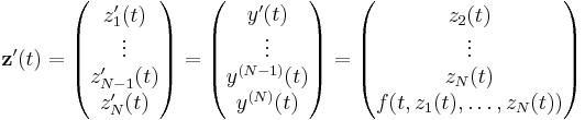
$\mathbf{z}'(t) = \begin{pmatrix} z_1'(t)\\ \vdots\\ z_{N-1}'(t)\\ z_N'(t) \end{pmatrix} = \begin{pmatrix} y'(t)\\ \vdots\\ y^{(N-1)}(t)\\ y^{(N)}(t) \end{pmatrix} = \begin{pmatrix} z_2(t)\\ \vdots\\ z_N(t)\\ f(t,z_1(t),\ldots,z_N(t)) \end{pmatrix}$

This is a first-order system in the variable $\mathbf{z}(t)$ and can be handled by Euler's method or, in fact, any other scheme for first-order systems.

Example

Given the differential equation $y'=y$ and the initial point $y(0)=1$ , we would like to use the Euler method to approximate $y_3$ using step size $h=1$ .

The Euler method is

$y_{n%2B1} = y_n %2B hf(t_n,y_n). \qquad \qquad$

so first we must compute $f(t_0, y_0)$ . This simple differential equation depends only on $y$ , so we need only worry about inputting the values for $y$ .

$f(y_0)=1. \qquad \qquad$

By doing the above step, we have found the slope of the line that is tangent to the solution curve at the point $(0,1)$ . Recall that the slope is defined as the change in $y$ divided by the change in $t$ , or $\operatorname{d}y/\operatorname{d}t$ .

The next step is to multiply the above value by the step size $h$ .

$h \cdot f(y_0) = 1 \cdot 1 = 1. \qquad \qquad$

Since the step size is the change in $t$ , when we multiply the step size and the slope of the tangent, we get a change in $y$ value. This value is then added to the initial $y$ value to obtain the next value to be used for computations.

$y_0 %2B hf(y_0) = y_1 = 1 %2B 1 \cdot 1 = 2. \qquad \qquad$

The above steps should be repeated to find $y_2$ and $y_3$ .

$y_2 = y_1 %2B hf(y_1) = 2 %2B 1 \cdot 2 = 4 \qquad \qquad$

$y_3 = y_2 %2B hf(y_2) = 4 %2B 1 \cdot 4 = 8 \qquad \qquad$

Due to the repetitive nature of this algorithm, it can be helpful to organize computations in a chart form, as seen below, to avoid making errors.

$y_n$	$t_n$	$y'(t)$	$h$	$dy$	$y_{n%2B1}$
1	0	1	1	1	2
2	1	2	1	2	4
4	2	4	1	4	8

Error

The magnitude of the errors arising from the Euler method can be demonstrated by comparison with a Taylor expansion of y. If we assume that $f(t)$ and $y(t)$ are known exactly at a time $t_0,$ then the Euler method gives the approximate solution at time $t_0%2Bh$ as:

$y(t_0 %2B h) = y(t_0) %2B h f(t_0,y(t_0)) \, \qquad \qquad$

In comparison, the Taylor expansion in $h$ about $t_0$ gives:

$y(t_0 %2B h) = y(t_0) %2B h y'(t_0) %2B \frac{1}{2}h^2 y''(t_0) %2B O(h^3).$

Since we know that $y'=f(t,y)$ it follows that

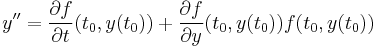
$y''={\partial f\over\partial t}(t_0, y(t_0)) %2B {\partial f\over\partial y}(t_0, y(t_0)) f(t_0, y(t_0))$

This, along with $f(t_0, y(t_0))$ can be inserted into the Taylor expansion in $h$ about $t_0$ .

$y(t_0 %2B h) = y(t_0) %2B h f(t_0, y(t_0)) %2B \frac{1}{2}h^2[{\partial f\over\partial t}(t_0, y(t_0)) %2B {\partial f\over\partial y}(t_0, y(t_0)) f(t_0, y(t_0))] %2B O(h^3).$

The error introduced by the Euler method is given by the difference between these equations:

$\frac{1}{2}h^2 [{\partial f\over\partial t}(t_0, y(t_0)) %2B {\partial f\over\partial y}(t_0, y(t_0)) f(t_0, y(t_0))] %2B O(h^3).$

For small $h$ , the dominant error per step, or the local truncation error, is proportional to $h^2$ . To solve the problem over a given range of $t$ , the number of steps needed is proportional to $1/h$ so it is to be expected that the total error at the end of the fixed time, or the global truncation error, will be proportional to $h$ (error per step times number of steps). Because the global truncation error is proportional to $h$ , the Euler method is said to be first order. This makes the Euler method less accurate (for small $h$ ) than other higher-order techniques such as Runge-Kutta methods and linear multistep methods.

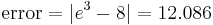
As stated in the introduction, decreasing the step size can help to make the approximation more accurate and decrease the error between the two curves. The error to three decimal places for the example in the above section (with step size $h=1$ )is the following:

$\text{error} = |e^3 - 8| = 12.086 \qquad \qquad$

When the step size is changed to $h=0.1$ our $y_3$ value becomes $17.449$ . The error, then, for step size $h=0.1$ is the following:

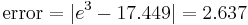
$\text{error} = |e^3 - 17.449| = 2.637 \qquad \qquad$

Although the error has decreased, our approximation is still not particularly accurate. In addition, since the step size decreased with no change in the interval, the number of iterations has increased to thirty. While possible, it is no longer reasonable to do these computations by hand.

Error bound

As with other methods, there is a way for us to determine an error bound for a particular problem. The error bound on the global error is given by^[1]:

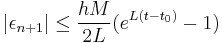
$|\epsilon_{n%2B1}| \le \frac{hM}{2L}(e^{L(t-t_0)}-1) \qquad \qquad$

where $h$ is the step size, $M$ is the upper bound on the second derivative of $y$ on the given interval (which must be estimated), and $L$ is the Lipschitz constant.

If the error bound is computed, it can be seen, once again, that if small error is desired, the step size $h$ must be very small.

For instance, let us calculate the step size required for global truncation error to be $\epsilon_{n%2B1}=0.01$ , assuming a maximum value for the second derivative of $M=10$ , a Lipschitz constant of $L=1$ , and $t$ from zero to four. Using the equation given, we obtain the following:

$\frac{2L}{M(e^{L(t-t_0)}-1)}|\epsilon_{n%2B1}|\le h \qquad \qquad$

$\frac{2}{10(e^{(4)}-1)}|0.01|\le h \qquad \qquad$

$h \le 0.0037314721 \qquad \qquad$

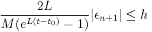
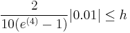
which means that h must be smaller than the above to get the desired error or less, and 4/h, or about 1072 iterations will need to be completed to do so. The large number of steps, and thus high computation cost, supports the use of alternative, higher-order methods such as Runge–Kutta methods or linear multistep methods.

Numerical stability

The Euler method can also be numerically unstable, especially for stiff equations. This limitation—along with its slow convergence of error with h—means that the Euler method is not often used, except as a simple example of numerical integration. The instability can be avoided by using the Euler–Cromer algorithm.

References

Ascher, Uri M.; Petzold, Linda Ruth. Computer methods for ordinary differential equations and differential-algebraic equations. 1998. SIAM. ISBN 0898714125

^ Simple Euler method and its modifcations

External links

Euler's Method for O.D.E.'s

Numerical integration

First order methods	Euler method · Backward Euler · Semi-implicit Euler · Exponential Euler

Second order methods	Verlet integration · Velocity Verlet · Crank–Nicolson method · Beeman's algorithm · Midpoint method · Heun's method · Newmark-beta method · Leapfrog integration

Higher order methods	Runge–Kutta methods · List of Runge–Kutta methods · Linear multistep method